Recently I’ve been doing a lot of CTF-styled crypto problems, where encryption schemes are purposefully flawed so that an attacker can break them and recover a “flag”. This led me to the question: how are attacks mounted against more “secure” ciphers that aren’t misused in some way? How were ciphers like FEAL (Fast data Encipherment ALgorithm) attacked and subsequently broken?
In these posts, I’ll look at one of the two most powerful and common techniques — linear cryptanalysis. Originally discovered by Mitsuru Matsui in 1992, linear cryptanalysis is a known ciphertext/plaintext attack (where the attacker has access to a large number of ciphertext-plaintext pairs). I’ll be following Howard M. Hey’s tutorial on linear and differential cryptanalysis, with a few more detailed diagrams that help illustrate the concepts — check that out if you haven’t already!
To illustrate how linear cryptanalysis works, we first need to build ourselves a basic yet somewhat resistant cipher — here, we’ll use a Substitution-Permutation Network (SPN).
Substitution-Permutation Networks
Substitution-Permutation Networks perform encryption by repeatedly applying substitutions and permutations over multiple rounds while mixing in the key; some famous examples of this design include DES (Data Encryption Standard) and AES (Advanced Encryption Standard). Let’s look at each of these components in more detail.
Substitution
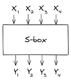
The substitution step is performed through something called an “S-box” — it takes in a block of bits and substitutes it with a different block (based on some fixed mapping).
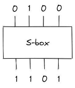
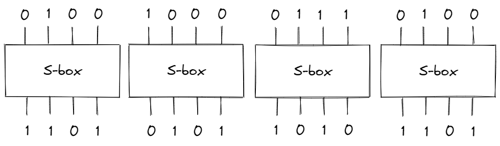
In the S-box above, the block of bits 0100 (8 in hex) produces a different block 1101 (D in hex). To apply the substitution step on longer inputs, we can divide the data into 4-bit blocks. For example, if the input was 0100100001110100 (4874 in hex), we would have:
Ideally, there shouldn’t be a relationship between the input bits and the outputs bits, but we’ll soon see how we can approximate S-boxes with linear functions.
Permutation
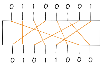
The permutation portion is what the name suggests — a block of bits is permutated by a “P-box”, according to some fixed table of indices.
Sample P-Box
| Input | 1 | 2 | 3 | 4 | 5 | 6 | 7 | 8 | | Output | 7 | 2 | 4 | 1 | 6 | 8 | 3 | 5 |
For the sample P-box above, the 1st bit of the input is the 7th bit of the output, the 2nd bit of the input is the 2nd bit of the output, and so on. Visualizing this permutation:
Key-Mixing
The final step is to mix the key into each of these substitution-permutation rounds. Commonly, an initial key is used to generate multiple round keys (known as subkeys), which are XOR’ed against the input to the round. For example, a single round may look like:
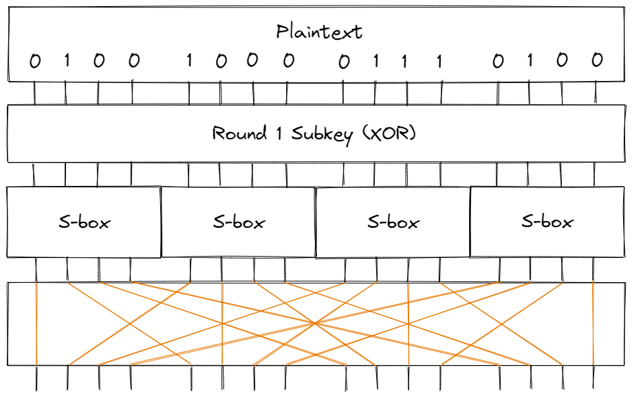
Our Cipher
The cipher we’ll work with consists of 4 rounds based on the diagram above; in the final round, we’ll skip over the permutation step since it doesn’t add any practical security (an attacker can simply “un-permutate” the bits of the ciphertext).
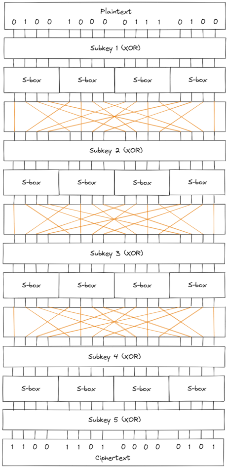
Using 5 distinct keys (each key being 16 bits), the cipher encrypts 16 bits of plaintext and produces 16 bits of ciphertext. Notice that a plain brute force attack on the keyspace would require $2^{5 \cdot 16} = 2^{80}$ encryptions, which is quite infeasible.
Implementation
An implementation of the cipher can be found here.
Linear Cryptanalysis
Linear cryptanalysis relies on approximating bits of the cipher through linear equations (since we’re working in GF(2), we’ll use XOR $\oplus$ operations). In other words, we’ll construct equations of the form:
$$X_{i_1} \oplus X_{i_2} \oplus \dots \oplus X_{i_u} \oplus Y_{j_1} \oplus Y_{j_2} \oplus \dots \oplus Y_{j_v} = 0$$
where $X$ represents input bits $([X_1, X_2, \dots])$ and $Y$ represents output bits $([Y_1, Y_2, \dots])$. With multiple linear expressions like these, we can deduce the bits of the key and effectively break the cipher.
Obviously, if equations like the one above hold with 100% probability, then the cipher is practically useless. Ideally, these linear equations should be accurate exactly half the time, preventing any information from being leaked. However, that’s rarely the case — our goal is to find linear equations that hold with either a high or low probability. A higher probability implies that the XOR of all the bits tends to be 0, while a lower probability implies the opposite (that the XOR of all the bits tends to be 1). To simplify things, we’ll introduce a term:
Bias refers to the amount a probability deviates from $\frac{1}{2}$. Specifically, the probability bias is $p - \frac{1}{2}$, and thus the bias is bounded by $[-\frac{1}{2}, \frac{1}{2}]$. The greater the magnitude of bias for a linear equation ($| p - \frac{1}{2}|$), the more effective linear cryptanalysis will be.
Now, the question arises: how can we find linear equations with significant bias (that hold with a higher or lower probability than $\frac{1}{2}$)?
Looking at the different components of the cipher, we see that key mixing doesn’t affect the magnitude of a bias. If a key bit is 0 and then XOR’ed to the data, it doesn’t change the probability that a linear equation holds true; otherwise, if a key bit is 1, then the bias simply flips and changes sign. Similarly, the permutation step only changes the order of the bits; we can easily update the indices of the bits in a linear equation to match the p-box permutation, so that the equation still has the same probability. The only nonlinear aspect of the cipher is the S-box, which takes in 4 bits and produces 4 seemingly unrelated bits. However, we can create linear approximations for the S-box and combine them together to represent the entire cipher with linear expressions.
Linear approximations for S-box
Let’s say the S-box has input bits $[X_1, X_2, X_3, X_4]$ and output bits $[Y_1, Y_2, Y_3, Y_4]$; our goal is to create linear expressions involving those variables and to calculate their bias.
Since the S-box involves only 8 variables, we can brute-force all possible linear expressions and keep track of how often they hold true.
| $X_1$ | $X_2$ | $X_3$ | $X_4$ | $Y_1$ | $Y_2$ | $Y_3$ | $Y_4$ | $X_1 \oplus X_4$ | $Y_1$ | $X_1 \oplus X_4 \oplus Y_1$ | ||
|---|---|---|---|---|---|---|---|---|---|---|---|---|
| 0 | 0 | 0 | 0 | 1 | 1 | 1 | 0 | 0 | 1 | 1 | ||
| 0 | 0 | 0 | 1 | 0 | 1 | 0 | 0 | 1 | 0 | 1 | ||
| 0 | 0 | 1 | 0 | 1 | 1 | 0 | 1 | 0 | 1 | 1 | ||
| 0 | 0 | 1 | 1 | 0 | 0 | 0 | 1 | 1 | 0 | 1 | ||
| 0 | 1 | 0 | 0 | 0 | 0 | 1 | 0 | 0 | 0 | 0 | ||
| 0 | 1 | 0 | 1 | 1 | 1 | 1 | 1 | 1 | 1 | 0 | ||
| 0 | 1 | 1 | 0 | 1 | 0 | 1 | 1 | 0 | 1 | 1 | ||
| 0 | 1 | 1 | 1 | 1 | 0 | 0 | 0 | 1 | 1 | 0 | ||
| 1 | 0 | 0 | 0 | 0 | 0 | 1 | 1 | 1 | 0 | 1 | ||
| 1 | 0 | 0 | 1 | 1 | 0 | 1 | 0 | 0 | 1 | 1 | ||
| 1 | 0 | 1 | 0 | 0 | 1 | 1 | 0 | 1 | 0 | 1 | ||
| 1 | 0 | 1 | 1 | 1 | 1 | 0 | 0 | 0 | 1 | 1 | ||
| 1 | 1 | 0 | 0 | 0 | 1 | 0 | 1 | 1 | 0 | 1 | ||
| 1 | 1 | 0 | 1 | 1 | 0 | 0 | 1 | 0 | 1 | 1 | ||
| 1 | 1 | 1 | 0 | 0 | 0 | 0 | 0 | 1 | 0 | 1 | ||
| 1 | 1 | 1 | 1 | 0 | 1 | 1 | 1 | 0 | 0 | 0 |
For example, the table above lists all possible values for the linear expression:
$$X_1 \oplus X_4 \oplus Y_1$$
In this case, the probability that the expression is equal to 0 is $\frac{4}{16} = \frac{1}{4}$, and hence the bias is $\frac{1}{4} - \frac{1}{2} = -\frac{1}{4}$. We can apply a similar process for all $2^8 = 256$ different expressions, and generate the table below:
Table 1. A linear approximation table for the S-box
The columns of this table represent the input bits, while the rows represent the output bits. Each value indicates the number of times a given linear equation holds true, subtracted by 8. For example, $$X_1 \oplus X_4$$ is represented as 1001 = 9, while $$Y_1$$ is represented as 1000 = 8. The value at (9, 8) is -4 in the table above, implying that $$X_1 \oplus X_4 \oplus Y_1$$ has a bias of $\frac{-4}{16} = -\frac{1}{4}$.
In other words, the expression $$X_1 \oplus X_4 \oplus Y_1$$ has a greater probability of being 1 rather than 0.
Approximating the entire cipher
To attack the complete cipher, we can combine multiple of these linear approximations to derive an equation involving plaintext bits and intermediate bits.
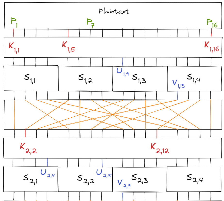
To simplify things, let’s introduce a few variable names first:
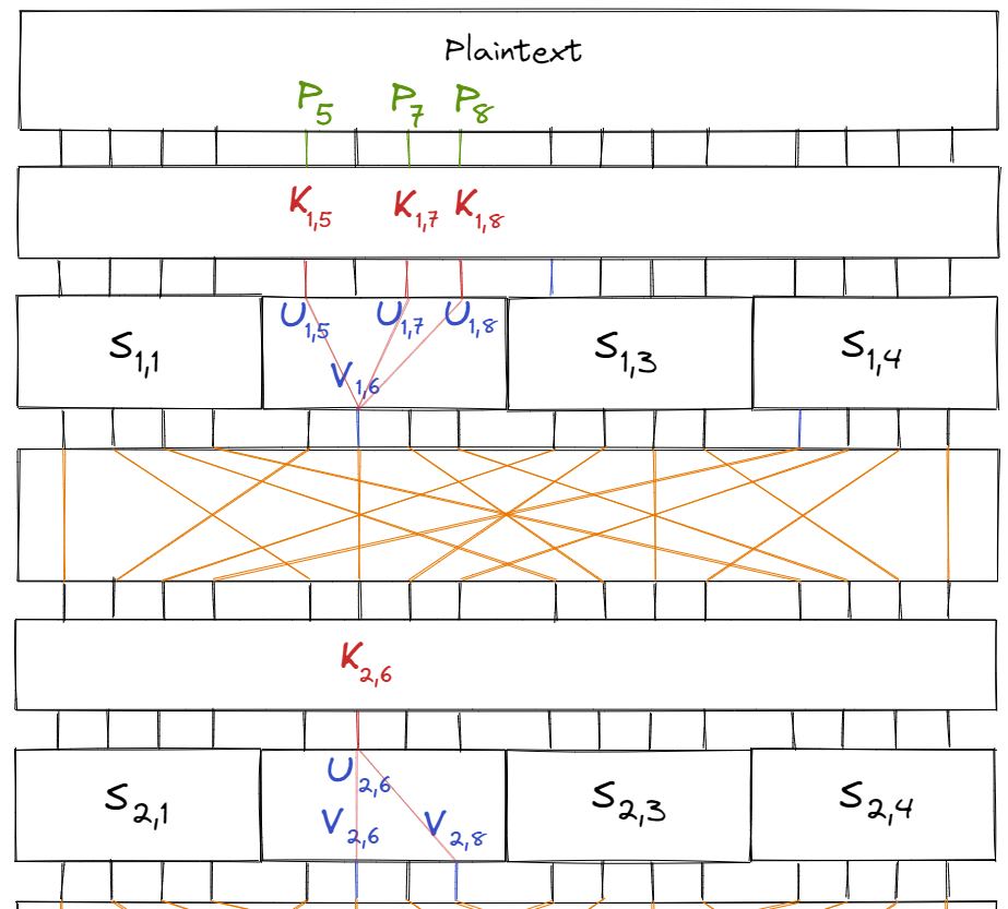
Let $S_{i, j}$ be the $j$‘th S-box of the $i$‘th round. Similarly, let $K_{i, j}$ be the $j$‘th key bit of the $i$‘th subkey and $P_i$ be the $i$‘th bit of the plaintext. Finally, let $U_{i, j}$ and $V_{i, j}$ be the $j$‘th input and output bits of round $i$’s S-box respectively.
Labelled in the diagram below:
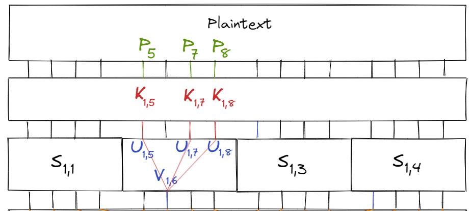
Consider the linear equation $$X_1 \oplus X_3 \oplus X_4 = Y_2$$ (for a S-box). According to Table 1, the equation holds true with probability $\frac{12}{16} = \frac{3}{4}$ and bias $\frac{1}{4}$ (see value of table at (B, 4)).
Additionally, we know that $U_{1, i} = P_i \oplus K_{1, i}.$ Combining all of this for the S-box $S_{1, 2}$, we have the equation:
$$\begin{aligned} V_{1, 6} &= U_{1, 5} \oplus U_{1, 7} \oplus U_{1, 8} \\ &= (P_5 \oplus K_{1, 5}) \oplus (P_7 \oplus K_{1, 7}) \oplus (P_8 \oplus K_{1, 8}) \end{aligned}$$
which holds true with $\frac{3}{4}$ probability.
We can apply a similar process to approximate the intermediate bits in later rounds. For example, consider the linear approximation $$X_2 = Y_2 \oplus Y_4$$ for the S-box $S_{2, 2}$, which holds with probability $\frac{1}{4}$. Then we can approximate $V_{2,6} \oplus V_{2,8}$ by:
$$\begin{aligned} V_{2, 6} \oplus V_{2, 8} &= U_{2, 6} \\ &= V_{1, 6} \oplus K_{2, 6} \\ &= (P_5 \oplus K_{1, 5}) \oplus (P_7 \oplus K_{1, 7}) \oplus (P_8 \oplus K_{1, 8}) \oplus K_{2, 6} \\ &= (P_5 \oplus P_7 \oplus P_8) \oplus (K_{1, 5} \oplus K_{1, 7} \oplus K_{1, 8} \oplus K_{2, 6}) \end{aligned}$$
Once again, we’ve expressed intermediate bits (of the second round) as a linear approximation of plaintext and subkey bits.
Continuing this one more time with the same linear approximation $$ Y_2 \oplus Y_4 = X_2$$ on the S-boxes $S_{3, 2}$ and $S_{3, 4}$, we get the two equations:
$$\begin{aligned} V_{3, 6} \oplus V_{3, 8} &= U_{3, 6} \\ V_{3, 14} \oplus V_{3, 16} &= U_{3, 14} \end{aligned}$$
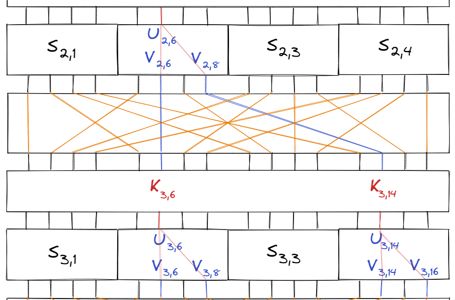
Furthermore, since $U_{3, 6} = V_{2, 6} \oplus K_{3, 6}$ and $U_{3, 14} = V_{2, 8} \oplus K_{3, 14}$, we can write:
$$\begin{aligned} (V_{3, 6} \oplus V_{3, 8} \oplus V_{2, 6} \oplus K_{3, 6}) \oplus (V_{3, 14} \oplus V_{3, 16} \oplus V_{2, 8} \oplus K_{3, 14}) &= 0 \\ (V_{3, 6} \oplus V_{3, 8} \oplus V_{3, 14} \oplus V_{3, 16}) \oplus (V_{2, 6} \oplus V_{2, 8}) \oplus (K_{3, 6} \oplus K_{3, 14}) &= 0 \end{aligned}$$
We know the value of $(V_{2, 6} \oplus V_{2, 8})$ from our earlier S-box approximations, so after substituting:
$$\begin{aligned} (V_{3, 6} \oplus V_{3, 8} \oplus V_{3, 14} \oplus V_{3, 16}) \oplus (P_5 \oplus P_7 \oplus P_8) \oplus (K_{1, 5} \oplus K_{1, 7} \oplus K_{1, 8} \oplus K_{2, 6}) \oplus (K_{3, 6} \oplus K_{3, 14}) &= 0 \end{aligned}$$
Now our expression has gotten quite complicated, but what it tells us is that we can approximate the value $$(V_{3, 6} \oplus V_{3, 8} \oplus V_{3, 14} \oplus V_{3, 16})$$ of the 3rd round through only plaintext and subkey bits.
Our final step is to approximate the bits right before the last round of S-boxes, and this occurs after one more subkey.
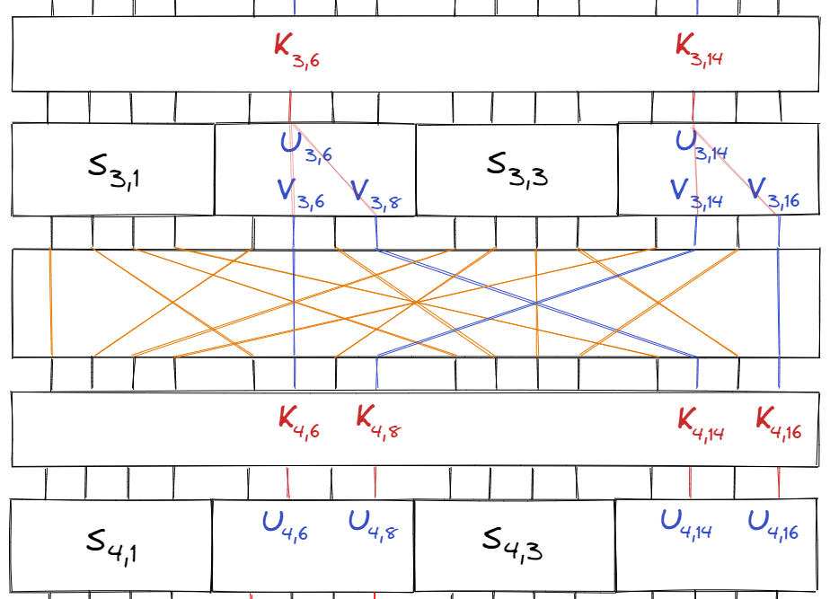
From the diagram above, we can see that:
$$\begin{align} U_{4, 6} &= V_{3, 6} \oplus K_{4, 6} \\ U_{4, 8} &= V_{3, 14} \oplus K_{4, 8} \\ U_{4, 14} &= V_{3, 8} \oplus K_{4, 14} \\ U_{4, 16} &= V_{3, 16} \oplus K_{4, 16} \end{align}$$
And substituting these variables into our previous equation one last time, we get:
$$(U_{4, 6} \oplus U_{4, 8} \oplus U_{4, 14} \oplus U_{4, 16}) \oplus (P_5 \oplus P_7 \oplus P_8) \oplus \Sigma_K = 0$$
where $$\Sigma_K = (K_{1, 5} \oplus K_{1, 7} \oplus K_{1, 8} \oplus K_{2, 6} \oplus K_{3, 6} \oplus K_{3, 14} \oplus K_{4, 6} \oplus K_{4, 8} \oplus K_{4, 14} \oplus K_{4, 16}).$$
Since $\Sigma_K$ is a fixed value, the expression $$(U_{4, 6} \oplus U_{4, 8} \oplus U_{4, 14} \oplus U_{4, 16}) \oplus (P_5 \oplus P_7 \oplus P_8)$$ will hold with a bias (we’ll find the exact probability in the following post).
So, now we have an equation that relates the plaintext bits and the intermediate bits of the second-to-last round.
Looking Ahead
In the next post, I’ll explain how we can use the above expression to determine the final round’s subkey (and subsequently the entire key), in addition to providing code and exploring some other aspects of this linear cryptanalysis attack.
Resources
- A Tutorial on Linear and Differential Cryptanalysis by Howard M. Heys
- An explanation of SP Networks by Computerphile